Some calculations are too slow to run as often as you want them. A finite element model of a part can take minutes or hours per design. An optimiser that wants to try ten thousand designs cannot wait for ten thousand of those. So you run the real model a few times, fit something fast to the results, and let the optimiser query the fast thing. That fast thing is a surrogate model, also called a metamodel or response surface.
The catch is that the surrogate only knows what the few real runs told it. This note shows how much that matters, on a beam small enough to check by hand.
The expensive model, pretended
A rectangular aluminium cantilever, length L = 200 mm, width b = 20 mm, with F = 20 N at the tip and E = 70 GPa. The tip deflection as a function of thickness t is:
δ = F L³ / (3 E I), with I = b t³ / 12, so δ = 4 F L³ / (E b t³) = 457.1 / t³ mm, with t in mm
That formula is instant, which is what makes it a good test. Pretend it is a slow simulation. We can afford four runs, at t = 4, 6, 8 and 10 mm, which give δ = 7.14, 2.12, 0.89 and 0.46 mm.
Surrogate one: a quadratic
The textbook response surface is a quadratic polynomial, δ ≈ a + b t + c t², fitted by least squares. On these four points it comes out as δ ≈ 22.73 − 5.081 t + 0.2869 t². It looks reasonable on the four runs. Here is how it does elsewhere:
| t, mm | True δ, mm | Quadratic, mm | Error |
|---|---|---|---|
| 2 (outside) | 57.1 | 13.7 | −76% |
| 5 | 3.66 | 4.49 | +23% |
| 9 | 0.63 | 0.24 | −62% |
| 12 (outside) | 0.26 | 3.07 | +1061% |
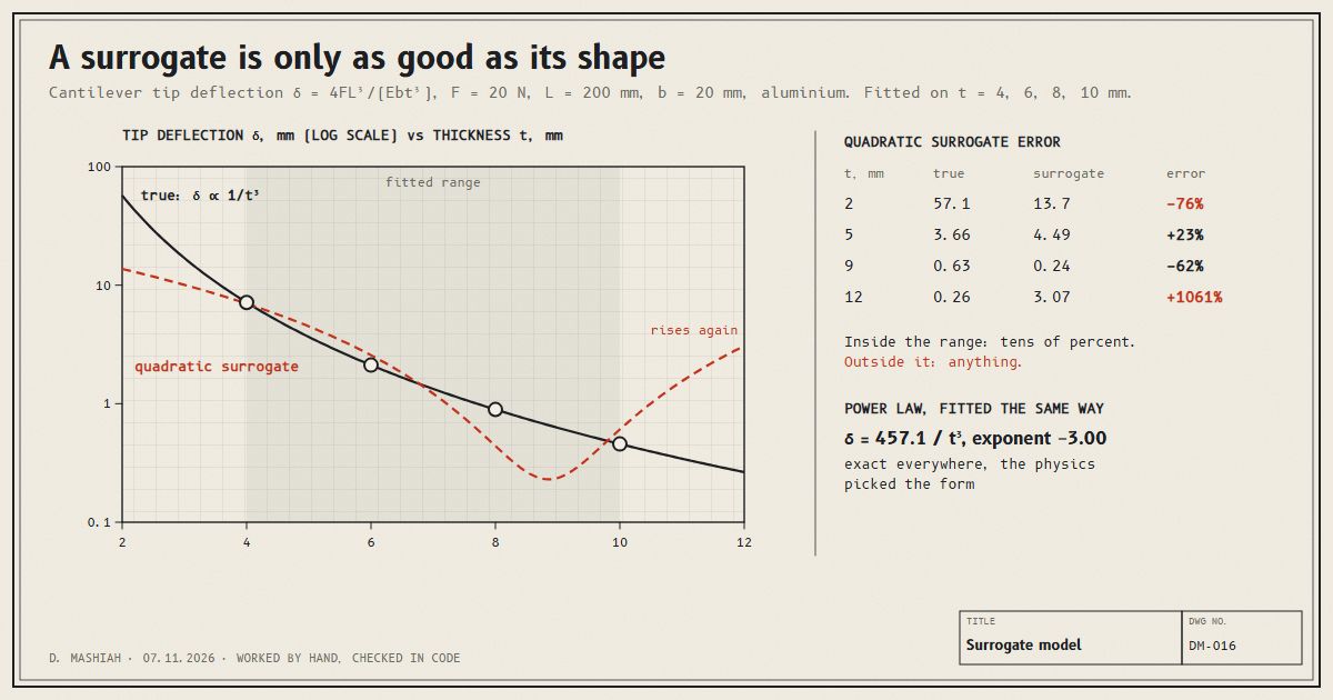
Inside the range it is off by up to 66 percent, at t = 8.7 mm. Outside, at 12 mm, it is off by a factor of 11.6. And it has a minimum at t = 8.85 mm, so past that point it predicts that a thicker beam deflects more. No beam does that. An optimiser looking for the stiffest design would be steered by a feature that is purely an artefact of the polynomial.
Surrogate two: the right shape
Now fit a power law, δ ≈ a · tᵏ, to the same four runs. Taking logs makes it a straight line, log δ = log a + k log t, which is an ordinary least squares fit. It gives a = 457.1 and k = −3.00. That is the exact formula, recovered from four points.
Same data, same fitting method, same number of runs. The only difference is that the power law has the shape the physics has. Stiffness of a bending beam goes with t³, and a power law can say that. A quadratic cannot, so it bends itself to pass near four points and gets everything between and beyond them wrong.
This is a clean example, with no noise and a known answer. Real surrogates are built where the answer is not known, which is the reason for building them. But the lesson carries: knowledge of how the system scales is worth more than more flexible fitting.
Inside and outside the range
The table has two kinds of error. Between the runs, the surrogate interpolates, and the error is bounded by how well its shape matches. Beyond them, it extrapolates, and nothing bounds the error at all. The quadratic goes from tens of percent inside to over a thousand percent just 2 mm outside.
Machine-learning surrogates such as neural networks and Gaussian processes are far more flexible than a quadratic, but they share this. They are trustworthy near the data they were trained on and have no particular reason to be right away from it. The same failure, worked with five numbers, is in the out-of-distribution note. It is also what my own research measures: where machine-learning surrogates of mechanical metamaterials fail on unit-cell shapes they were not trained on.
How to tell whether to trust one
- Hold runs back. Score the surrogate on real runs it was not fitted on, the same way as a train/test split. Four points fitted and four points scored tells you nothing.
- Check physical sense. A surrogate that says a thicker beam bends more, or a negative mass, is wrong however good its error score is.
- Know the range. Record what inputs it was built on, and treat any query outside them as unanswered.
- Use the uncertainty if it gives one. A Gaussian process reports how unsure it is at each point, and that number grows away from the data. Adding a real run where it is most unsure is how many surrogate-based optimisers choose their next simulation.
References
- Forrester, A. I. J., Sóbester, A. and Keane, A. J. Engineering Design via Surrogate Modelling: A Practical Guide. Wiley, 2008.
- Queipo, N. V. et al. Surrogate-based analysis and optimization. Progress in Aerospace Sciences 41(1), 2005.