R², the coefficient of determination, is a comparison with a baseline. The baseline is the dumbest prediction possible: the mean of the data, for every point. R² asks what share of the baseline's squared error your model removes.
The formula, with numbers
Eight points, x = 1 to 8, with y = 4.0, 3.5, 8.1, 6.9, 12.4, 10.2, 15.8, 14.1. The mean of y is 9.375.
SS_tot, the total sum of squares, is the squared miss of the baseline: Σ (y − mean)². Here it is 144.6.
SS_res, the residual sum of squares, is the squared miss of your model. A least-squares line through these points is y = 1.66 + 1.71x, and its squared misses add to 21.2.
R² = 1 − SS_res / SS_tot = 1 − 21.2 / 144.6 = 0.854
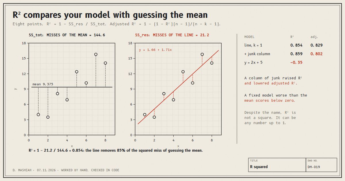
So the line removes 85 percent of the squared error of guessing the mean. That is all R² says. It does not say the predictions are within 15 percent, or that the line is the right model, or that it will do as well on new data.
R² can be negative
The name suggests a square, so it cannot be below zero. It can. Take a model that was not fitted to these points, say y = 2x + 5, from some other dataset. Its squared misses here add to 195.7, more than the baseline's 144.6:
R² = 1 − 195.7 / 144.6 = −0.35
A negative R² means the model is worse than predicting the mean every time. It cannot happen for a least-squares line scored on its own training data, because the mean is one of the lines it could have chosen. It happens all the time on test data, which is where it matters. It is worked through as a real failure in the out-of-distribution note, and in the cross-validation note, where the same model scores 0.80 or −0.67 depending on how the data was split.
More inputs always help, on paper
Add a second input to the model: a column z = 3, 7, 1, 5, 8, 2, 6, 4, which is just the numbers 1 to 8 shuffled and has nothing to do with y. Fit y = a + b·x + c·z by least squares.
R² goes up, from 0.854 to 0.859. It always does, or stays the same, when you add an input to a least-squares fit on its training data, because the fit can always set the new coefficient to zero and do no worse. With enough junk columns, R² climbs toward 1 on data the model has simply memorised.
Adjusted R²
Adjusted R² charges for each input. With n points and k inputs:
adjusted R² = 1 − (1 − R²) · (n − 1) / (n − k − 1)
| Model | k | R² | Adjusted R² |
|---|---|---|---|
| Line in x | 1 | 0.854 | 1 − 0.146 × 7 / 6 = 0.829 |
| x plus the junk column z | 2 | 0.859 | 1 − 0.141 × 7 / 5 = 0.802 |
The junk column raised R² and lowered adjusted R². The penalty factor (n − 1) / (n − k − 1) grew from 7/6 to 7/5, and the small gain in fit was not enough to pay for it. An input has to earn its place.
Adjusted R² is a correction on training data, though, not a replacement for testing. The honest check is still the score on data the model has not seen, from a held-out test set or cross-validation.
Reading R² in practice
- It is relative to the spread of the data. The same model error gives a high R² on data that varies a lot and a low one on data that barely varies. Compare R² only between models on the same data.
- It says nothing about size in units. For that, report an error in the target's own units, such as RMSE or MAE, next to it.
- Training R² flatters. Always say which data it was computed on.
- Below zero is not a bug. It is the model doing worse than the mean, and it is worth knowing.