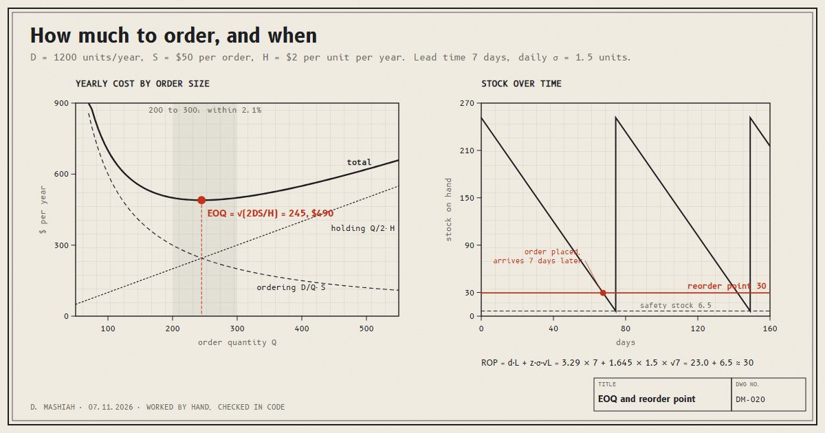
Order a lot at once and you pay to hold it: storage, capital tied up, things that spoil or go out of date. Order a little at a time and you pay for every order: the paperwork, the delivery, the receiving. The economic order quantity, EOQ, is the order size where those two costs balance.
The numbers below are a made-up product, chosen to be easy to check.
The setup
- Demand D = 1200 units a year, steady.
- Ordering cost S = $50 for each order placed, whatever its size.
- Holding cost H = $2 per unit per year, for every unit sitting in stock.
Order Q units at a time and you place D / Q orders a year, costing (D / Q) · S. Stock runs from Q down to zero and back, so on average Q / 2 units sit on the shelf, costing (Q / 2) · H. The total is the sum.
The square root
The total is lowest where the two costs are equal. Setting (D / Q) · S = (Q / 2) · H and solving for Q gives:
EOQ = √(2 D S / H) = √(2 × 1200 × 50 / 2) = √60000 = 245 units
At 245, ordering costs $245 a year and holding costs $245 a year, $490 in total. That is about 4.9 orders a year, one every 75 days.
The flat bottom
This is the part worth remembering. Here is the total yearly cost at other order sizes:
| Order size Q | Ordering | Holding | Total | Above the best |
|---|---|---|---|---|
| 100 | $600 | $100 | $700 | +42.9% |
| 150 | $400 | $150 | $550 | +12.3% |
| 200 | $300 | $200 | $500 | +2.1% |
| 245 | $245 | $245 | $490 | 0 |
| 300 | $200 | $300 | $500 | +2.1% |
| 400 | $150 | $400 | $550 | +12.3% |
Anything from 200 to 300 is within 2.1 percent of the best. You can round to a full pallet or a supplier's case size and lose almost nothing.
The same flatness protects you from bad inputs. Ordering cost is hard to pin down. Say it is really $100, not $50. The true EOQ is then 346, costing $693 a year. Keep ordering 245 and you pay $735, just 6.1 percent more, after getting an input wrong by a factor of two. The square root shrinks any error in S, D or H, so doubling S moves the EOQ by only 41 percent, and the flat bottom absorbs most of what is left.
When to order: the reorder point
An order takes time to arrive. Say the lead time is L = 7 days. Demand is 1200 / 365 = 3.29 units a day, so 3.29 × 7 = 23.0 units go out while you wait. Order when stock falls to 23 and, on an average week, the delivery arrives as the shelf empties.
Half the time demand runs above average and the shelf empties first. The cover for that is safety stock. If daily demand varies with standard deviation σ = 1.5 units, demand over 7 days varies by σ · √L = 1.5 × √7 = 3.97 units. Holding z of those as a buffer gives:
reorder point = d · L + z · σ · √L
| Chance of not running out in a cycle | z | Safety stock | Reorder point |
|---|---|---|---|
| 90% | 1.28 | 5.1 | 28 |
| 95% | 1.645 | 6.5 | 30 |
| 99% | 2.33 | 9.3 | 32 |
So: order 245 units whenever stock falls to 30. Each step from 90 to 95 to 99 percent costs more safety stock than the step before, because the normal distribution's tail thins out.
Where EOQ misleads
- It assumes steady demand. Seasonal or trending demand needs a forecast first, and the method has to match the shape.
- It assumes the history is demand, not sales. On days that sold out, sales understate demand, and both D and σ come out too low. That is the censored demand problem.
- It assumes stock keeps. For things that spoil or go out of date, such as flowers, food or newspapers, a unit left over is a loss, not a holding cost, and the right model is the newsvendor model.
- It ignores quantity discounts and truck sizes. Those are handled by checking the cost at each price break, which the flat bottom usually makes painless.