A demand forecast is a guess at how much people will want, made early enough to act on: to order stock, plan a shift or book a truck. The methods range from one line of arithmetic to large models. The simple ones are worth understanding first, because they fail in ways you can see, and the large ones fail in the same ways less visibly.
This note runs five of them on one made-up series and scores each the same way.
The data and the test
Twelve weeks of demand, rising with some noise: 20, 22, 19, 24, 23, 26, 25, 27, 30, 28, 31, 33.
Each method forecasts one week ahead using only the weeks before it, for weeks 5 to 12. That is eight forecasts each, and every one is made without seeing the week it predicts. That matters: a forecast scored on data it was built from scores better than it will ever do for real.
Each is scored by MAE, the average size of the miss, and by bias, the average miss with its sign kept. Error is forecast minus actual, so a negative bias means too low.
Five methods
- Mean of history. Forecast the average of every week so far. It treats all weeks as equally relevant.
- Naive. Forecast last week's value. It throws away everything older.
- Moving average. Forecast the average of the last 3 weeks. A compromise between the two.
- Simple exponential smoothing. Keep a level L, and after each week move it part of the way toward what happened: L = α · y + (1 − α) · L. With α = 0.5 it moves halfway. The forecast is L.
- Holt's method. The same, plus a trend T that is smoothed the same way, with its own weight β. The forecast is L + T. Here α = 0.5 and β = 0.3, starting from L = 20 and T = 2, the first two weeks.
| Method, weeks 5 to 12 | MAE | Bias |
|---|---|---|
| Mean of history | 4.81 | −4.81 |
| 3-week moving average | 2.38 | −2.38 |
| Simple exponential smoothing, α = 0.5 | 2.31 | −2.31 |
| Naive, last week | 2.13 | −1.13 |
| Holt, α = 0.5, β = 0.3 | 1.39 | +0.11 |
What the numbers say
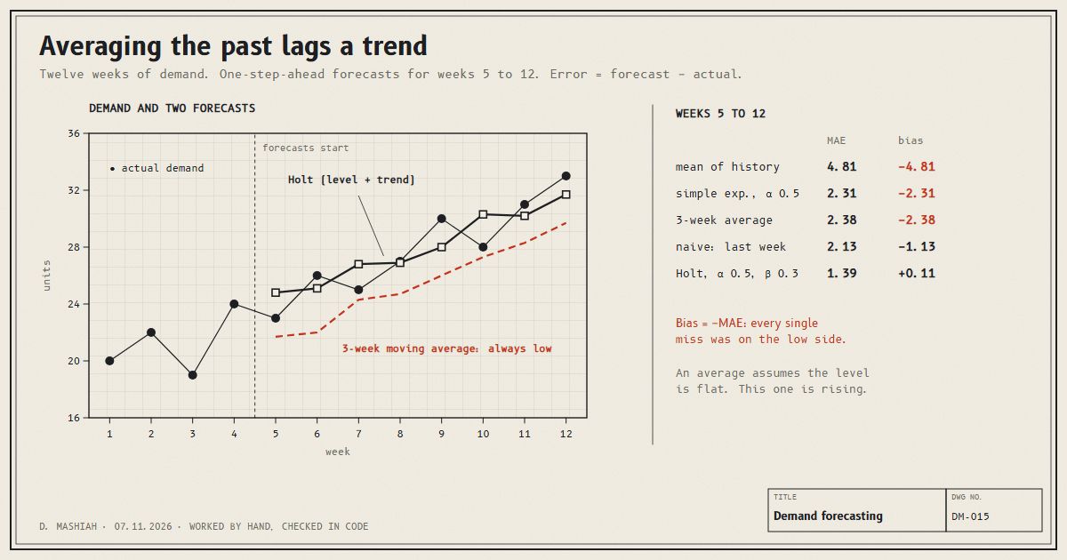
Look at the first three rows. Bias equals minus MAE exactly. That only happens when every single error is negative: all eight forecasts too low, every time. These methods average past weeks, and on a rising series the past is always smaller than the present. The more history an average includes, the further behind it falls, which is why the mean of all history is worst.
Naive does better because it uses only last week, so it is only one week behind. Holt's method does best, MAE 1.39 against 2.31 for exponential smoothing without a trend, a 40 percent cut, and its bias is close to zero. It is the only one of the five that has a term for the thing the data is actually doing.
One warning about Holt's score. Its two weights matter. With α = 0.3 and β = 0.1 it overshoots instead: MAE 1.74, bias +1.72. In practice the weights are fitted on the history, before the test weeks, not picked by looking at which pair scores best on them. Picking them by the test score is the same mistake as choosing a random seed by its result.
The shape decides the method
None of these methods is good or bad in general. Each assumes a shape. An average assumes the level is flat and the wiggles are noise. Holt assumes a level that drifts in a straight line. Demand with a weekly or yearly cycle needs a seasonal term on top, which is what Holt–Winters adds. On flat demand, the average would win and Holt would chase noise.
So the first step is not choosing a model. It is plotting the history and asking whether it is flat, trending, seasonal, or affected by things you know about, like promotions and holidays. The bias column is the quickest check that a method's assumption is wrong: a bias that stays on one side, week after week, means the method is missing a pattern.
The same holds across items as well as over time. On one Walmart store in the M5 data, a machine-learning model beat a moving average on the steady items and lost by about 10 percent on the intermittent and lumpy ones, which is worked through in the note on value added by demand class.
Two things the method cannot fix
The history has to be demand, not sales. On a day that sold out, sales stop at the stock you had, and every method above will learn that people wanted less than they did. That is worked through in the censored demand note.
And a forecast is not an order. The forecast says what demand is likely to be. How much to stock depends on what it costs to be short against what it costs to be over, which is the newsvendor model. A good forecast with the wrong order is still the wrong amount of stock.